Original Post

今天我们来看读者@王静萍 的问题。她问到投资中「卖」的问题：
收益多少了卖？卖的时间点怎么把握？用定投可以避开「买」的择时，那「卖」依据什么呢？
在之前的文章什么时候卖出中，我说过有三种情况我会卖出。

第一种，买错了（或者说逻辑变了）。这种情况下不管买入后是盈利还是亏损，我都会果断卖出。

第二种，变贵了。好公司还需要好价格，如果股票的价格已经远远超过了它的内在价值，我会选择卖出。

第三种是有更好的标的。如果发现了更好的投资标的，而手头有没有额外的现金，就可以卖出现在的去买入更好的标的。需要注意的是，你究竟有没有能力去判断两个不同的公司未来预期收益率的差别。我做过很多这样的交易，最后成功的概率并不高。

今天这个问题，我邀请到谭昊老师来回答。

谭老师从投资者的底层逻辑出发，认为卖出并不是一个孤立的动作，应该和你的投资系统相匹配。

相信你看完后，会豁然开朗。

这是个好问题，有句谚语说得好，会买的是徒弟，会卖的是师傅。

但是要准确的回答这个问题，却不能从问题本身入手。好比我经常说的，不能在同一层楼解决这层楼的问题，而必须上一层楼。上一层楼干什么呢？欲穷千里目更上一层楼。上楼，是为了要从系统的角度看问题。

你要理解卖出，就不能光看卖出这个孤立的动作，卖出当然不是一个孤立的点，而是整个交易系统中的一个环节。就像一串珍珠项链的中间一粒珍珠，你不能脱离它的上下文去看它。

所以我们要谈卖出的问题，首先，要明白卖出的动作要跟你的交易系统的底层逻辑相匹配。

为了更清楚地说明这个问题，我举一个充满争议的例子你就明白了，那就是止损。

投资中到底要不要止损？关于这一点迄今为止没有定论，支持和反对的人都能各自举出一百条理由，以及无数的血泪史和鲜活的案例。

可以说按照这样的方式去争论，再过一百年也不会有一个明确的结果出来。因为止损这个行为本身是没有对错的。

止损卖出

止损这个动作要不要做？

取决于它是否跟你的买入动作匹配，跟你的整个交易系统的底层逻辑匹配。当匹配的时候它就是对的，不匹配的时候它就是错的。

比如说你买入的理由是趋势来了，一个股票的价格站上了20日均线，你按照趋势交易系统的逻辑进行了买入操作。那么当价格跌破了20日均线，这个趋势买入逻辑已经不成立了，难道你不应该止损吗？既然你是以趋势买入的，就应该在趋势不存在的时候止损，这不是天经地义的吗？

但是如果你买入的理由是价值就不同了。

比如一只股票，你认为它内在价值有10块钱，你在价格8块钱的时候买入了，过了一段时间价格跌到了7块钱。价格被低估的幅度不是更大了吗？按照你的价值低估的买入逻辑，你应该更大幅度的买入才对，这个时候止损不是荒唐吗？

当然这里不是说价值投资者不能止损，这里是说价值投资者不能按照价格的跌幅来止损，不能用形态走坏了之类的标准来止损，那叫牛头不对马嘴。如果你是按价值方法买入的，那么只有在这个公司基本面走坏，你的价值买入逻辑不存在的时候，你才应该止损。

止损是卖出的一种情境，如果你把这个情境背后的理论模型搞清楚了，你就能正确的理解卖出这个行为了。

让我再简单的总结一下，止损这个行为本身没有对错好坏，你必须把它放到你的交易系统的全局中去理解。如果止损这个动作跟你的买入动作相匹配，跟你的交易系统的底层逻辑相匹配，那就是对的，否则就是错的。

看到这里，相信你已经准备好了，接下来我们来谈更广义的卖出。

什么时候应该卖出呢？

正确的答案是，你先搞明白，你的交易系统的底层逻辑是什么？然后根据这个系统去匹配相应的卖出策略。

一般来说卖出有三种情形，分别称之为止损卖出，止盈卖出以及失去性价比优势卖出。

止损的情形前文已经讲过了，这里不重复了。

止盈卖出

我们来看看止盈。

同样的我们在底层把所有的交易系统分为两大类型，一种是趋势类的，一种是价值类的，我们分开讲。

在趋势类的系统中， 你的买入理由是趋势来了，你盈利的法宝是截断亏损让利润奔跑。所以，在趋势跟踪系统中一般不设目标位卖出，不是说你认为主观上认为股票涨到了多少钱就卖出，因为那个时候趋势可能还在。

在趋势系统中用的比较多的止盈卖出，是动态跟踪止盈。就是股票从最高位回落一个百分比，你认为趋势被破坏了，此时卖出。

而在价值类的交易系统中，你买入的理由是股票的价格被低估，那么相对应的卖出的理由应该是股票价格被高估。还是举刚才那个例子，假如你经过测算，如果一只股票的内在价值是10块钱，你8块钱买入了。那么当这支股票涨到15块的时候，因为它的价格明显高估，你就把它卖出了。但具体多少比例算是高估，取决于每个人对公司基本面的认识以及对市场情绪面的把握，这个不能一概而论。

以上讲的止盈卖出。

失去性价比优势卖出

还有第三种卖出情形是，因为丧失了足够的性价比优势而卖出，这种情形基本是在价值类的交易系统中使用，因为趋势类的系统不看性价比，只看趋势本身。

这个方法其实很多的价值类的投资大师都在用，比如巴菲特、邓普顿等等。

你会同时关注市场上的很多股票，当你持有的某一只A公司的股票经过股价的上涨，它的价格已经高估了，但是接下来还会不会上涨，其实你是不知道的。高估的幅度达到多少应该卖出，其实是没有一个固定标准的。

但是这个时候出现了另外一家公司B公司，它的股价却明显处于大幅低估的状态，这个时候你卖出a公司，转而买入b公司，相当于把自己的资产向性价比高的地方集中，这是符合价值投资的底层逻辑的。

事实上，这可能是一个典型的价值投资者最常用的卖出方式，因为你可能永远都不知道高估多少应该卖出，这个是非常困难的。但是在不同的公司中间做性价比的比较，卖出明显高估的，买入明显低估。这个切换的操作是相对容易的。

而邓普顿在这个基础上更进了一步，他说，你不但要这么做，而且要在全球范围内这么做。所以他曾经去抄底日本，抄底韩国，直至在日本股市赚了很多钱之后，又抛出日本的股票转而投资其他地区。基于这个性价比的比较逻辑。

至于说定投应该什么时候卖出，你用上面我讲的方法去判断，就一目了然了。

目前市场上绝大部分的定投策略都是价值类的定投，就是买入相对低估的，性价比高的指数，既然是价值类的定投，那么卖出就参照价值逻辑来卖出就对了。

而一些定投体系，事实上已经把丧失性价比优势卖出这一条，内嵌到了定投策略当中。

如果是这样的自带策略的体系，那么理论上你不需要再去主动卖出。如果是自己定投指数基金，那么你就参照价值类交易系统的匹配原则，去制定卖出策略。

卖出的科学与艺术

让我再简单总结一下关于卖出的科学与艺术。

卖出基本上可以分为三种情形，止损卖出，止盈卖出和丧失性价比优势的卖出。

卖出的单一动作是无法评判好坏对错的，它必须跟你的整个交易系统的底层逻辑相匹配。我们用最质朴的方法，把所有的交易系统归为趋势类和价值类两大类型，你再去匹配你的卖出策略，就能豁然开朗。

我的思考

1. 价值投资中，如何判断一个股票的真实价值？
2. 如何比较不同股票的性价比优势？本质上和问题1相同。当一个股票走强时，市场几乎会持续看涨这支股票，个人并没有足够多的信息去判断股价到底有没有超越真实的价值。

Introduction

A central problem in graph theory is the shortest path problem which is to find the shortest path between two nodes (vertices) in a graph so that the sum of the weight of its constituent edges is minimum. There are four variations of the shortest path problem namely, single-source shortest path (SSSP), breadth-first search (BFS), all-pairs shortest path (APSP), and single-source widest path (SSWP). Many algorithms are in use today which solve this problem. Some of the most popular algorithms are Dijkstra’s algorithm, Bellman-Ford algorithm, A* search algorithm, and Floyd-Warshall algorithm. These algorithms can be applied to undirected as well as directed graphs. Interesting research has been done on this problem due to its many useful real-world applications like road networks, community detection, currency exchange, logistics, electronic design, etc. In this project, we focused on the parallelization of three algorithms - Dijkstra’s algorithm, Bellman-Ford algorithm and Floyd-Warshall algorithm and analyze the speedups against sequential implementations.

Literature Review

Parallelization of the classical shortest path algorithms can be done in several ways. Some of the ways have been discussed by B. Popa et al. [1] Another approach to parallelize Dijkstra’s algorithm has been discussed by A. Crauser et al. [2]
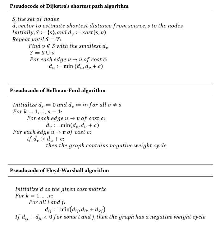
To discuss parallelizing the classical algorithms, we discuss the main idea of the three algorithms we used in our experiment, namely: Dijkstra’s algorithm, Bellman-Ford algorithm and Floyd-Warshall algorithm in the following.
Dijkstra’s algorithm finds the shortest path from a single source and at each step, it finds the minimal distant node, tries to find the shortest paths to other nodes using the recently found shortest node. This algorithm does not consider negative weights and thus cannot be used in a graph with negative weights.
Bellman-Ford algorithm also finds the shortest path from a single source. However, at each step in contrary to Dijkstra’s algorithm, this algorithm updates each node’s distance from the source by the observing the edges. Bellman-Ford algorithm can detect negative weight cycles in a graph and also can be used in a graph with negative weights.
Floyd-Warshall algorithm finds all pair shortest path and does that by observing each node at a time and update paired shortest distances if the node can contribute. This algorithm also can be used in a graph with negative weights.
The pseudocodes of Dijkstra’s algorithm, Bellman-Ford algorithm and Floyd-Warshall algorithm are given in Figure 1 below.
Figure 1. Pseudocode of Dijkstra’s algorithm, Bellman-Ford algorithm and Floyd-Warshall algorithm

The running time and space complexity of the algorithms are given in Table 1 below:

Our Solution

The three algorithms we chose for our experiment are classic and they have been used in numerous applications. If we observe the time complexity of the algorithms, we see all three are having significant calculation part i.e. arithmetic integrity. According to the roofline model, the more arithmetic intensity an algorithm has, the more performance gain can be achieved using parallelization while increasing the data set. Therefore, we used parallelization to gain performance. For parallelization we used OpenMP.

OpenMP is an API for writing multi-threaded applications. The API supports C/C++ and Fortran on a wide variety of architectures. OpenMP provides a portable, scalable model for developers of shared memory parallel applications.
OpenMP is an abbreviation for Open Multi-Processing. It is comprised of three primary API components:

• Compiler Directives
• Runtime Library Routines
• Environment Variables

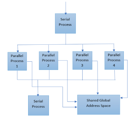
OpenMP uses the fork-join model of parallel execution. All OpenMP programs begin as a single process: the master thread. The master thread executes sequentially until the first parallel region construct is encountered. The master thread then creates a team of parallel threads. The statements in the program that are enclosed by the parallel region construct are then executed in parallel among the various team threads. When the team threads complete the statements in the parallel region construct, they synchronize and terminate, leaving only the master thread. The number of parallel regions and the threads that comprise them are arbitrary.

Because OpenMP (Fig. 2) is a shared memory programming model, most data within a parallel region is shared by default. OpenMP provides a way for the programmer to explicitly specify how data is “scoped” if the default shared scoping is not desired.
Figure 2. OpenMP thread Model

Experimental Setup

For the experimental setup, we used four machines. Three of the machines were personal laptops. The fourth one is a computer node of Farber cluster which is the University of Delaware’s second Community Cluster. Farber cluster uses distributed-memory running on Linux operating system (Cent OS). A summary of these machines can be seen in the following table.

To see the compiler effect, we compile the performance using two different compilers: GCC and ICC (intel compiler), both of which are available on Farber.

The data sets used in our project are fake maps generated with script containing different number of nodes. We chose the number node to be 20, 100, 500, 1000 to see the effect of map size. For all the running time reported in this project, it is an average of running the same program on the same machine for 5 times.

Results

Serial Running Time

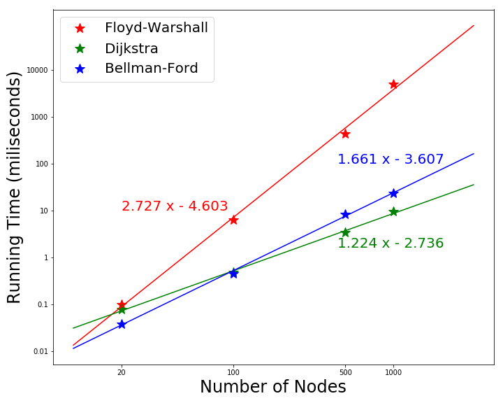
The sequential running time is plotted in Fig. 3. This is the running time of the graph with 1000 nodes on machine 3. From the figure we can see that Floyd Warshall algorithm is the slowest one and scales close to $O(V^3)$. As the nodes increases, Dijkstra’s algorithm is more efficient: $O(V^2)$ becomes smaller than $O(VE)$ as the number of edge gets larger.
Figure 3. Scale of running time with increasing nodes in the graph

Effects of Compiler: GCC vs. ICC

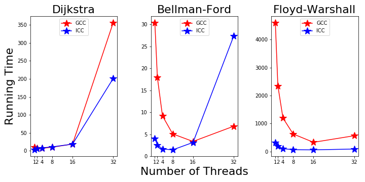
On farber, we compiled all three algorithms with ICC and GCC. The running time on the 1000 node graph is shown in Fig. 4. The ICC significantly outperformed GCC before we go over 8 threads. For Bellman-Ford and Floyd-Warshall algorithms, the difference is as much as one order in magnitude. This means GCC is not optimized as ICC for the intel CPU. Another interesting result is that the speed up with more threads is more prominent with GCC, as their running time become comparable with 16 threads.
Figure 4. GCC and ICC compiler

Parallel Running Time on Machine 1: OS X

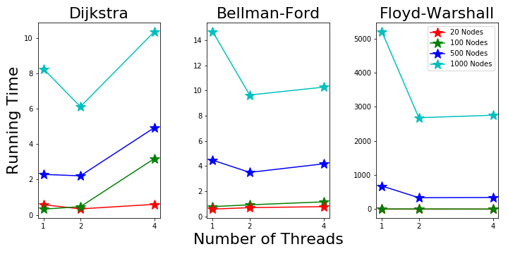
On the macbook pro with OS X, we see decreasing running time from 1 to 2 threads. More speed up is achieved with more nodes with parallelization.
For all the three algorithms, there’re no improvement from 2 to 4 threads. This is possibly because it only has 2 physical cores and the 4 logical threads are not so efficient.
Figure 5. Parallel Running Time on Machine 1

Parallel Running Time on Machine 2: Windows

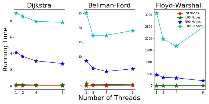
Machine 2 is a Windows laptop with 2 intel i7 processors and 4 threads. From Fig. 6 we can see Dijkstra’s running time keeps decreasing as more threads are used. The 4 thread mode shows good performance, which is better than the macbook pro.
Figure 6. Parallel Running Time on Machine 2

Parallel Running Time on Machine 3: Ubuntu

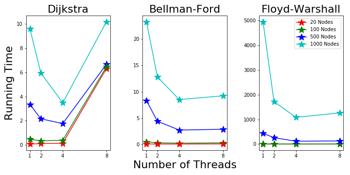
Machine 3 has 4 physical cores and 8 total threads. The results in Fig. 7 show good speed up going from 1 to 4 threads. However, the 8 threads mode is not very helpful.
Figure 7. Parallel Running Time on Machine 3

Parallel Running Time on Machine 4: Cent OS

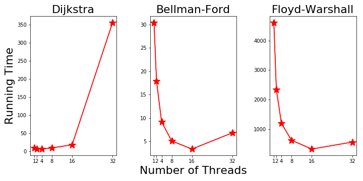
The personal laptops have limited number of CPU cores. But for Farber clusters, it has 20 cores each node, making it good to explore the speed up with more cores. So on machine 4 we focus on the speed up with more threads and just run the three algorithms on one graph with 1000 nodes. The results running with programs compiled with GCC are plotted in Fig. 8. The Dijkstra’s running time start to increase after 4 threads and goes to very high with 32 threads. Further investigation is needed to find out the reasons. The other two algorithms show decreasing running time up to 16 threads. The 32 threads’ running time start to increase as there’re only 20 physical cores.
Figure 8. Parallel Running Time on Machine 4

Discussion

Amdahl’s Law and Roofline Model

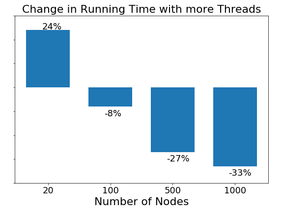
A general trend in all machines and all algorithms is that ast the number of node increases, the speed up effect becomes more prominent. The average change in running time from one to two threads for graphs with different nodes is shown in Fig. 9. The more nodes in the graph, the more prominence of scale up with more threads. This could be related to Amdahl’s law, which says taht performance improvement to be gained from using some faster mode of execution is limited by the fraction of the time the faster mode can be used. With more nodes in the graph, a larger fraction of the code can be parallelized.
Figure 9. Speed up with respect to graph size

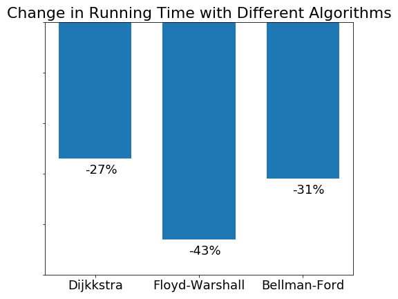
Roofline model tells us that the more arithmetic intensity an algorithm has, the more performance gain can be achieved using parallelization. Arithmetic intensity is the ratio of the total floating point operations to the total data movement. In our problem, the three algorithms has different arithmetic intensity, we would expect different speed up with the three algorithms. Fig. 10 shows the change in running time with different algorithms when going from 1 thread to 2 threads. Floyd-Warshall’s algorithm shows the largest decrease in running time, which is as expected as it has the largest arithmetic intensity with running time scales like $O(v^3)$. Our results correctly demonstrate the Roofline model.
Figure 9 Speed up with respect to different algorithms

Applications

There are many applications for shortest path algorithm. To name a few:

1. Shortest Path Algorithms are used in google maps to find the short path between the source and destination. We can also say it as it is used to find the direction between two physical locations. Google maps uses A* algorithm to do the same.
2. Shortest path algorithm is used in IP routing to find the Open shortest path first.
3. It is also used in telephone networks.
4. Used to find arbitrage opportunities in currency exchange problem.

Finding Arbitrage Opportunities in Currency Exchange Problem.

For this problem we use Bellman Ford Algorithm. Bellman ford is used because the graph can have negative edges and this algorithm can be used to find if the graph has any negative cycles. For this problem we use negative log of the exchange rates to change as the weights of the edges. This done to change the problem from maximization problem to minimization problem. The Table 4. gives details about the exchange rates between the 6 different currencies. If the graph has any negative cycles indicates that this currency exchange has arbitrage opportunities. We can use backtracking to find between which currency exchange pair this arbitrage opportunity exists. Arbitrage opportunity results from a pricing discrepancy among the different currencies in the foreign exchange market.

Conclusions

In conclusion, parallelization definitely reduces the time cost compared to the sequential run time of the three algorithms. Doing this project brought into light that the speedup of thread-level parallelization depends on the machine as well as the operating system. The results produced demonstrates Amdahl’s law and the Roofline model. Not only were the benefits of parallelization exposed but to see the algorithms being applied to a useful application like currency exchange was quite interesting.

Future Work

Further investigation can be done on the parallelization of Dijkstra’s algorithm and seek to improve the runtime for more number of threads. It would also be fascinating to apply these effective algorithms for more applications like the GPS system, electronic design, telephone networks, etc. The shortest path problem is certainly worth exploring due to its countless implementations.

All the code and data sets can be found in the GitHub repository as listed in [9].

References

[1]. Popa, B., & Popescu, D. (2016, May). Analysis of algorithms for shortest path problem in parallel. In Carpathian Control Conference (ICCC), 2016 17th International (pp. 613-617). IEEE.

[2]. Crauser, A., Mehlhorn, K., Meyer, U., & Sanders, P. (1998, August). A parallelization of Dijkstra’s shortest path algorithm. In International Symposium on Mathematical Foundations of Computer Science (pp. 722-731). Springer, Berlin, Heidelberg.

[3]. Bellman-Ford algorithm in Parallel and Serial - GitHub link
https://github.com/sunnlo/BellmanFord

[4]. Dijkstra’s Shortest Path Algorithm
https://people.sc.fsu.edu/~jburkardt/cpp_src/dijkstra/dijkstra.cpp

[5]. Floyd, R. W. (1962). Algorithm 97: shortest path. Communications of the ACM, 5(6), 345.

[6]. Floyd Warshall Algorithm
https://engineering.purdue.edu/~eigenman/ECE563/ProjectPresentations/ParallelAll-PointsShortestPaths.pdf

[7]. Bellman-Ford Algorithm Tutorial
https://www.programiz.com/dsa/bellman-ford-algorithm

[8]. Shortest Path Algorithms Tutorial https://www.hackerearth.com/practice/algorithms/graphs/shortest-path-algorithms/tutorial

[9]. https://github.com/Zhiqiang-UD/CISC662

About Scrapy

Scrapy is a free and open source web crawling framework , written in Python. Originally designed for web scraping, it can also be used to extract data using API. or as a general purpose web crawler. It is currently maintained by Scrapinghub Ltd. , a web scraping development and services company.

Architecture Overview

Data Flow

The following diagram shows an overview of the Scrapy architecture with its components and and outline of data flow (red arrows).
architecture
The data flow is controlled by the execution engine and goes like this (as indicated by the red arrow):

1. The Engine gets the initial Requests to crawl from the Spiders.
2. The Engine schedules the Requests in the Scheduler and ask for the next Requests to crawl.
3. The Scheduler sends back the next Requests to the Engine.
4. The Engine send the Requests to the Downloader through the Downloader Middlewares (see process_request()).
5. Once the Downloader finishes the downloading it generates a Response and sends it back to Engine through the Downloader Middlewares (see process_response()).
6. The Engine sends the received Response to the Spiders for processing through the Spider Middleware (see process_spider_input()).
7. The Spiders processes the Response and returns the scraped Items and new Requests (to follow) to the Engine through the Spider Middleware (see process_spider_output()).
8. The Engine sends the scraped Items to Item Pipelines, then send the processed Requests to the Scheduler and ask for the next possible Requests to crawl.
9. The process repeats (from step 1) until there are no more requests from the Spiders.

Components

Scrapy Engine

The engine controls the data flow between all components and triggers events when certain action occurs. See Data Flow for more details.

Scheduler

The Scheduler receives the request from the engine and enqueues them for feeding them back to engine later when requested.

Downloader

The Downloader is responsible for fetching web pages from the Internet and feeding them back to the engine.

Spiders

Spiders are custom classes written by the user to parse responses and extract scraped items from them or additional requests to follow. Each spider is used for one (or a series of) specific webpage.

Item Pipelines

The Item Pipelines is responsible for processing the extracted items from the spiders. Typical tasks include cleansing, validation and persistence (like stoing the item in a database)

Downloader Middleware

Downloader Middleware is a specific hook between the Engine the the Downloader and processes requests when pass from the Engine to the Downloader and responses that pass from Downloader to the Engine. It provides a simple mechanism to extend Scrapy by inserting user defined code, like automatic replace user-agent, IP, etc.

Spider Middleware

Spider Middleware is a specific hook between the Engine and the Spider and processes spider input (response) and output (items and request). It also provides a simple mechanism to extend Scrapy functions by using user-defined code.

Process to Create a Scrapy Project

Create Project

First you need to create a Scrapy project. I’ll use the England Premier League website as an example. Run the following command:

scrapy startproject EPLspider

The EPLspider directory with the following content will be created:

EPLspider/
├── EPLspider
│   ├── __init__.py
│   ├── __pycache__
│   ├── items.py
│   ├── middlewares.py
│   ├── pipelines.py
│   ├── settings.py
│   └── spiders
│       ├── __init__.py
│       └── __pycache__
└── scrapy.cfg

The content of each file:

• EPLspider/: Python module of the project, in which code will be added.
• EPLspider/items.py: item file of the project.
• EPLspider/middlewares.py: middlewares file of the project.
• EPLspider/pipelines: pipelines file of the project.
• EPLspider/settings: settings file of the project.
• EPLspider/spiders/: directory with spider code.
• scrapy.cfg: configuration file of the Project.

Start with the First Spider

Spiders are classes that you define and that Scrapy uses to scrape information from a website (or a group of websites). They must subclass scrapy.Spider and define the initial request to make, optionally how to deal with links in the pages, and how to parse the downloaded page content to extract data.

This is our first Spider, EPL_spider.py, saved in the directory EPLspider/spiders/.

from scrapy.spiders import Spider

class EPLspider(Spider):
    name = 'premierLeague'
    start_urls = ['https://www.premierleague.com/clubs']

    def parse(self, response):
        club_url_list = response.css('ul[class="block-list-5 block-list-3-m block-list-2-s block-list-2-xs block-list-padding dataContainer"] ::attr(href)').extract()
        club_name = response.css('h4[class="clubName"]::text').extract()
        club_stadium = response.css('div[class="stadiumName"]::text').extract()
        for i,j in zip(club_name, club_stadium):
            print(i, j)

Run the Spider

Run the following command in the project folder:

scrapy crawl premierLeague

The club name and stadium of all clubs from the England Premier League will be printed out.

Summary

In this tutorial we show the overall architecture of Scrapy and show its basics with a demo. In the next tutorial, we’ll extend this simple spider program to get more detailed information about the England Premier League, i.e. clubs, players, managers, and match information, etc.

Welcome to Hexo! This is your very first post. Check documentation for more info. If you get any problems when using Hexo, you can find the answer in troubleshooting or you can ask me on GitHub.

Quick Start

Create a new post

$ hexo new "My New Post"

More info: Writing

Run server

$ hexo server

More info: Server

Generate static files

$ hexo generate

More info: Generating

Deploy to remote sites

$ hexo deploy

More info: Deployment

Delete post

1. Delete the post under source/_post folder
2. Run hexo clean to delete the database (db.json) and assets folder
3. Run hexo generateto generate the new blog without your deleted post
4. Run hexo deploy to deploy your blog

Add local images

• Set post_asset_folder: true in _config.yml.
• Add an npm package npm i -s hexo-asset-link
• Use syntax ![Alt Text](Post-Asset-Folder/image-name.png) for images in ./source/_posts/Post-Asset-Folder/image-name.png

More info: Asset Folders, Local Images with Markdown